Modes of Information Flow
In the previous post of the series, I introduced Information Theory with the concepts of entropy, mutual information, and transfer entropy. Now, using the same framework and moving a little deeper into the development of information theory measures, I will present the Modes of Information Flow developed by James et al. (2018). These modes try to establish a differentiation in the kind of information that is transferred from one variable to another. We can think about the modes of information as a decomposition of the amount of transfer entropy we studied in the previous post of this blog.
Modes of Information Flow
We already described that information measures were created based on probabilistic terms. We noticed that the probabilistic nature of information makes it account for different correlations between variables; in fact, the analogous relationship between entropy and variance and mutual information and covariance was already introduced. These conditions generate a good starting point to look for mechanisms that explain how the information is transferred between variables.
Information flow is the movement of information from one agent or system to another. Historically, this kind of flow has been measured using the time-delayed mutual information:
\[ I[ X_{-1}:Y_0] \tag{1} \]
The equation (1) presents the mutual information between \( X \)’s past \( (X_{-1}) \) and \( Y \)‘s present \( (Y_0) \). Here, the information flow is captured by the time-delayed structure. However, it fails to distinguish between exchanged and shared information due to common history. In other words, how much of the information of \( Y_0 \) depends on its history. To overcome the problem of the shared dependence present in the time-delayed mutual information, Schreiber (2000) proposed the transfer entropy.
\[ I[ X_{-1}:Y_0 | Y_{-1}] \tag{2} \]
Introducing the condition on \( Y \)‘s past transfer entropy excludes the influence of the common history on \( Y_0 \). Unfortunately, this is not enough to distinguish the different mechanisms for the information flow from \( X \) to \( Y \).
Considering the previous limitations, James et al. (2018) proposed that information flow from time series \( X \) to \( Y \) can take three qualitatively different modes. First, intrinsic flow, which is when the past behavior of \( X \) directly predicts the present of \( Y \) while the past of \( Y \) doesn’t give any information about \( Y \). Second, shared flow occurs when the present behavior of the time series \( Y \) can be inferred either by the past of \( X \) or the same \( Y \). Third, synergistic flow is when the past of both time series \( X \) and \( Y \) are each independent of \( Y \)‘s present, but if we combine them, they become predictive of \( Y \). In Figure 1, we can observe examples of the three modes of information flow.
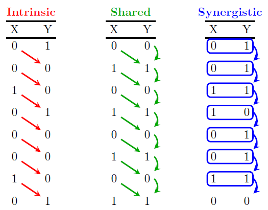
Figure 1: Modes of information flow. “Modes of information flow”, by R. G. James, B. D. Masante Ayala, B. Zakirov, and J. P. Crutchfield, 2018, Arxiv
Let’s use emotions to present the elements in a basic example. According to Hareli and Rafaeli (2008), the process of communicated emotions can be described as an evolution of mutual influence between dyads. The dynamic starts when one component of the dyad expresses a particular emotion, and then the other component replies, expressing its own emotions, and from there, the process becomes dialectical. In this setting, the evolution of the emotional content in the conversation follows three possible alternatives: contagion when messages express the same emotion, complement when messages express similar emotions, and inference when the receiver tries to predict the sender’s mood. The model proposed by Hareli and Rafaeli clearly shows the existence of a flow of emotional information between the dyad. Let’s say we are interested in analyzing a conversation between Yvonne and Xavier. After reviewing each message, determining its emotional content, and creating the time series, we can determine, for example, measure the transfer entropy between them. But what if we want to know how much of the evolution of emotions during the conversation between Yvonne and Xavier was due to contagion, complement, or inference following Hareli and Rafaeli’s model? In this case, the modes of information flow are helpful. Intrinsic flow can measure the concept of contagion, which is the reproduction of the same emotion that a person was exposed to. Shared flow works with the idea of the receiver’s prediction considering the sender’s expression and their experience to infer emotions. Finally, synergistic flow can be analogous to complementary emotions. Obviously, the overlap between the modes of information and the model proposed by Hareli and Rafaeli is not perfect. Still, it gives a good proxy to understand the primary mechanism of emotional flow in the conversation between Yvonne and Xavier. Figure 2 shows a representation of the application of the modes of information to Yvonne and Xavier’s conversation.
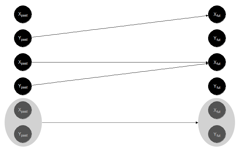
Figure 2
Analysis
Looking at the formula of time-delayed mutual information \( I[X_{-1}:Y_0] \) and considering the flows of Figure 1, it is possible to notice that time-delayed mutual information captures intrinsic and shared flows. On the other hand, with transfer entropy \( I[X_{-1}:Y_0|Y_{-1}] \) by conditioning on \( Y_{-1} \), the shared flow is excluded but intrinsic and synergistic flows are still captured. Therefore, as long as the intrinsic flow can be computed, the shared and synergistic flows can be derived using the time-delayed mutual information and transfer entropy.
The mathematical derivation of intrinsic mutual information escapes the scope of this blog, but if you are interested, you can look at the details in the paper (here). Here, I am going to give the intuitive idea that it is possible to define a slightly different past \( \overline{Y_{-1}} \) that I can condition on it to compute the intrinsic flow. The notation for the intrinsic flow is \( I[X_{-1}:Y_0 \downarrow Y_{-1}] \), and we obtain the different flow modes as follows:
- Intrinsic flow: \( I[X_{-1}:Y_0 \downarrow Y_{-1}] \)
- Shared flow: \( I[X_{-1}:Y_0] – I[X_{-1}:Y_0 \downarrow Y_{-1}] \)
- Synergistic flow: \( I[X_{-1}:Y_0 | Y_{-1}] – I[X_{-1}:Y_0 \downarrow Y_{-1}] \)

Figure 3
Another representation to clarify how the interaction between time series allows us to define the modes of information flow is presented in Figure 3. The image shows the interaction between the variables \( \overline{Y_{-1}} \), \( Y_{-1} \), \( X_{-1} \), and \( Y_0 \) as a markov chain. From the diagram:
- Time delayed mutual information: \( I[X_{-1}:Y_0] = a+b+c \)
- Transfer entropy: \( I[X_{-1}:Y_0 | Y_{-1}] = a \)
- Intrinsic flow: \( I[X_{-1}:Y_0 \downarrow Y_{-1}]=a+b \)
- Shared flow: \( (a+b+c) – (a+b) = c \)
- Synergistic flow: \( a – (a+b) = -b \)
It is important to note that the intrinsic mutual information is bound from the above by transfer entropy (conditional mutual information). Therefore, we conclude that \( b \leq 0 \).
Limitations
Like the case of transfer entropy, a fundamental assumption is that the time series used to compute the modes of information flow must be stationary.
The quantification of the intrinsic information flow is based on the cryptographic secret key agreement rate approximated with the intrinsic mutual information. Better upper bounds exist on the secret key agreement rate than on the intrinsic mutual information.
A Modes of Information Flow Application
For this example, I will use the same dataset and a slightly different problem from the application I shared in the Granger Causality post. Again, the objective is to analyze the relationship between online communicated emotions in the aftermath of a natural disaster. Using the modes of information flow, we want to know what emotions can be predicted by intrinsic, shared, or synergistic relationships with other emotions. The dataset collected information from Twitter in the aftermath of the earthquake that occurred in Southern California on July 5, 2019. To assess the emotion, each tweet was processed using the Natural Language Understanding tool provided by IBM Watson. This tool analyzes the text to assign a value from 0 to the presence of five emotions: sadness, anger, fear, disgust, and joy.
The procedure has the following steps:
- Setup: We load the packages needed to work on Python plus the dataset.
- Functions: Using Python packages, we create the functions to calculate the modes of information flow.
- Modes of information flow: We calculate the modes to identify the relationships between the five emotions studied.
- Figures: We create figures to have a visual perspective of the analysis.
References
Hareli, S., & Rafaeli, A. (2008). Emotion cycles: On the social influence of emotion in organizations. Research in Organizational Behavior, 28, 35–59. https://doi.org/10.1016/j.riob.2008.04.007
James, R. G., Ayala, B. D. M., Zakirov, B., & Crutchfield, J. P. (2018). Modes of Information Flow. ArXiv:1808.06723 [Cond-Mat, Physics:Nlin]. http://arxiv.org/abs/1808.06723
Schreiber, T. (2000). Measuring information transfer. Physical Review Letters, 85(2), 461