Transfer Entropy

In the fourth post of the series I am going to introduce an analytical tool called Transfer Entropy (TE) which is one of many measures developed thanks to the study of Information Theory. In short, Information theory studies the quantification, storage, and communication of information, it has its fundamental principles in the work published in 1948 by Claude Shannon titled “A mathematical theory of communication” and it has been a prolific scientific area ever since.

As I mentioned before TE is one of many measures within the study of Information Theory. It might be that the reader is not completely familiar with the reasoning of this theory so before defining the main method of this post I will do a brief introduction to two basic concepts of information theory: entropy and mutual information.

Entropy and Mutual information

It might be that you have heard the concept of entropy as a part of the study of thermodynamics. In that case, entropy is measure of the disorden in the system analyzed. For information theory, it is going to be necessary that you forget for a moment the previous definition because the idea of entropy proposed by Claude Shannon is slightly different. Professor Shannon was interested in measuring how much information a message conveyed so he thought about information in terms of probability. If an event is very likely to happen, the information we obtain when it actually happens is not much, like when we stop feeling hungry once we ate a meal, the result is expected. But when rare events happen, like when you don’t feel hungry during many days, they convey a great deal of information because of the surprise they generate (Bossomaier et al., 2016). So finally Shannon conceived entropy as the average uncertainty of a random variable which he expressed mathematically as:

(1) $H(X) = - \sum_{x \in X} p(x) \log_{2} p(x)$

Where $X$ is discrete random variable and $p(x)$ is the probability mass function for $X$ . It is possible to observe that the term $\log_{2} p(x)$ measures the uncertainty which is zero when $p(x)=1$ (complete certainty means no entropy), and the term $p(x)$ creates the average for the random variable $X$ .

Now that we have the gist of what entropy is let’s examine the concept of mutual information. Entropy was defined a measure of uncertainty, therefore, it give us information of a random variable, for example the variable $X$ . The same way we can obtain the information from another variable, let’s say $Y$ , measuring its entropy. When both random variables $X$ and $Y$ are dependent it would be logic to suppose that some portion of the information we are able to calculate is shared between $X$ and $Y$ , that is the mutual information. More formally, mutual information -denoted $I(X;Y)$ – is the amount of shared information between $X$ and $Y$ , it is measure of their statistical dependence.

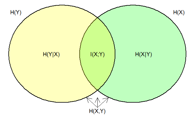
Figure 1

Using a Venn diagram figure 1 represent with different areas the information measures we can compute between two variables. Each full circle represents the measure of the entropy for each variable $H(X)$ and $H(Y)$ . The intersection area in the diagram is the amount of shared information between $X$ and $Y$ which is the definition of mutual information $I(X;Y)$ . Looking at the yellow portion in the left the sign $H(Y|X)$ represents the entropy of $Y$ once we know $X$ which is the conditional entropy of $Y$ given $X$ . Conversely, $H(X|Y)$ in the right side (green) is the conditional entropy of $X$ given $Y$ . Finally, because there exists dependence between the variables it is possible to define a joint probability distribution that allow us to compute the joint entropy $H(X,Y)$ .

Transfer Entropy

In information theory, information is defined in terms of uncertainty and this uncertainty is measured in terms of probability as defined in equation (1). We already reviewed the concepts of entropy and mutual information, looking at them it is possible to establish an analogous relation to the statistical measures of variance and covariance. Variance and entropy are measures of diversity, while covariance and mutual information establish the degree of association between variables. From this analogy we notice that the same as covariance or correlation, mutual information can’t imply a cause-effect relationship between variables, instead it is a symmetrical measure that reveals mutual influence.

Trying to address the idea of directionality using the association of variables, Schreiber (2000) proposed the concept of transfer entropy definying it as a conditional mutual information. The mutual information was conditioned using time-delay among three variables introducing markovian shielding and, therefore, directionality through temporal delay.

Figure 2

Let’s describe an example to help the understanding of the concept of TE. Following the same rationale that we have been using before let’s say that we are interested in measuring the information flow of emotions from Yvonne to Xavier. The process can be characterized as Yvonne_past $\longrightarrow$ Xavier_future. Figure 2 shows the process using Venn diagrams where the circles represent entropies and their intersection their mutual information. Figure 2 highlights in red the transfer entropy (information) of interest which flows from Yvonne expression of emotions (Yvonne_past) into Xavier’s (Xavier_future) expression after being exposed to Yvonne’s post while conditioning on the influence of Xavier’s previous emotions (Xavier_past), the condition on Xavier_past eliminates the effect of Xavier’s past on himself. Figure 3 shows a diagram of how information flows between variables.

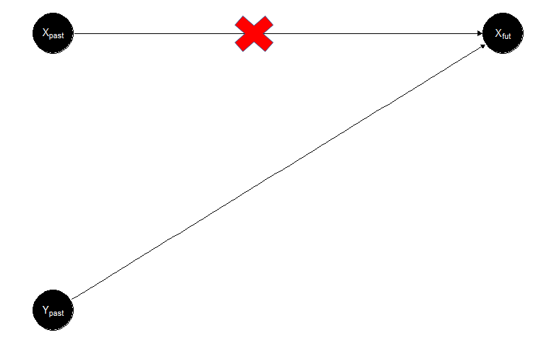
Figure 3

Analysis

In practice, it is possible to calculate the transfer entropy using the difference between conditional entropies.

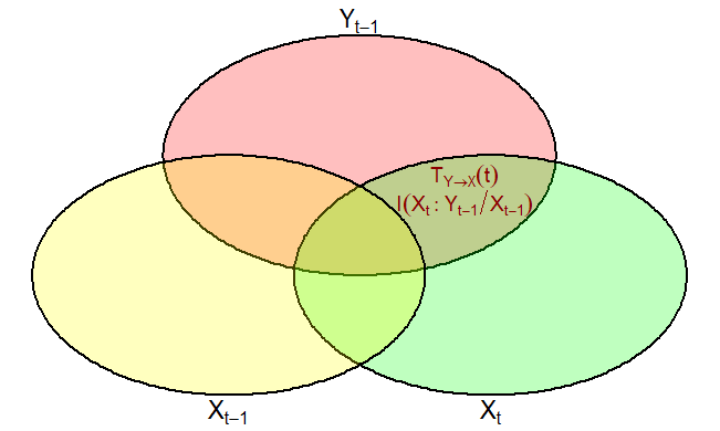
Figure 3

Figure 3 shows the information flow we are interested in, the transfer entropy, it can be matematically formulated as:

(2) $\begin{align*} T_{Y \to X} (t) &= I(X_{t} : Y_{t-1} | X_{t-1}) \\ &= H(X_{t}|X_{t-1}) - H(X_{t}|X_{t-1},Y_{t-1}) \end{align*}$

Replacing the definition of entropy given in (1) on equation (2) we obtain:

(3) $\begin{align*} T_{Y \to X} (t) &= \sum p(x_{t},x_{t-1},y_{t-1}) * \log_2 \frac{p(x_{t}|x_{t-1},y_{t-1})}{p(x_{t}|x_{t-1})} \end{align*}$

Transfer entropy can be considered as a non-parametric equivalent of Granger Causality with the difference that it also works for nonlinear categorical variables. In principle, the mutual information between both is symmetric (undirected), but the experimentally introduced time delay allows to establish directionality.

Limitations

One limitation is the assumption that the time series used to compute transfer entropy have to be stationary which requires that their mean and variance should be constant over time.

Another problem with the measure of transfer entropy is that it ignores the possibility of conditional dependence among variables. To overcome this issue researchers have proposed different Partial Information Decompositions (Finn & Lizier, 2018; James et al., 2018; Rauh et al., 2017; Williams & Beer, 2010). One of this decompositions will be the explanation of my next post.

A Transfer Entropy Example

In this section I will share an example of transfer entropy and time-delayed mutual information. We know that Transfer Entropy is time-delayed but conditioned $I(X_{t} : Y_{t-1} | X_{t-1})$ . Well time-delayed mutual information is not conditionated so it is defined as $I(X_{t} : Y_{t-1})$ . A more detailed explanation will be given in the next post but you will have its calculation in this example.

The example has the following steps:

Setup: We load the packages needed to work on Python.
Functions: Using the dit Python package we create the functions to calculate the time-delayed mutual information and transfer entropy.
Simulation: We create three different examples to calculate the time-delayed mutual information and transfer entropy.

View this gist on GitHub

References

Bossomaier, T., Barnett, L., Harré, M., & Lizier, J. T. (2016). An Introduction to Transfer Entropy: Information Flow in Complex Systems. Cham, Switzerland: Springer International Publishing; 2016.

Schreiber, T. (2000). Measuring information transfer. Physical Review Letters, 85(2), 461.

Shannon, C. E. (1948). A mathematical theory of communication. The Bell System Technical Journal, 27(3), 379–423. https://doi.org/10.1002/j.1538-7305.1948.tb01338.x

Transfer Entropy

Pablo M. Flores

ε-Machines

Modes of Information Flow

Instrumental Variables

Structural Causal Modeling

Granger Causality

Prediction and Explanation in Social Sciences: Introducing a Set of Useful Methods.