Step 1
First we load the packages needed to create the Structural Causal Modeland plot the DAG.
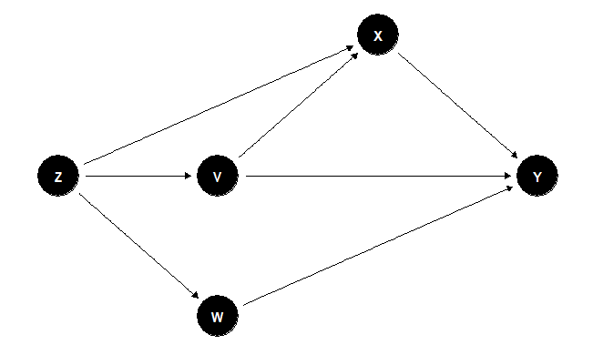
#We load the package dagitty to create the SCMlibrary(dagitty)#Definition of the DAGg <- dagitty("dag { Z [pos="1,1"] V [pos="2,1"] W [pos="2,0"] X [pos="3,2"] Y [pos="4,1"] Z -> X -> Y Z -> V -> Y Z -> W -> Y V -> X -> Y}")#We load the package ggdag to plot the DAGlibrary(ggdag)#Plot the DAGggdag(g) + theme_dag_blank()
Step 2
We ask to the software to get all the paths from X to Y
paths(g, "X", "Y")## $paths## [1] "X -> Y" "X <- V -> Y" "X <- V <- Z -> W -> Y"## [4] "X <- Z -> V -> Y" "X <- Z -> W -> Y" ## ## $open## [1] TRUE TRUE TRUE TRUE TRUEStep 3
From the previous result we can observe that there are four back-doorpaths from X to Y. Now we need to find the set of controls S which allowus to block all the back-door paths so we can obtain the real causaleffect of X on Y.
#Set SadjustmentSets(g, "X", "Y", type = "all")## { V, W }## { V, Z }## { V, W, Z }Here we got three different sets S_1 = {V,W}, S_2 = {V,Z}, and S_3 ={V,W,Z}. It is important to notice here that we don’t need to controlall the variables.
Step 4
We are going to illustrate the previous result by generating simulateddata for the model. Then using that data we are going to fit a model toobtain the estimates for the SCM.
#We load the package lavaan to simulate the data library(lavaan)#Simulated model (effects of exogenous variables are set to be non-zero)lavaan_model <- "Y ~ .7*X + .5*V + .3*W X ~ .5*Z + .6*V V ~ .4*Z W ~ .2*Z"#Data consistent with the simulated model with 1000 observationsset.seed(1234)g_tbl <- simulateData(lavaan_model, sample.nobs=1000)The previous code specifies a traditional SEM, which means that all thefunctions in the SCM are linear. Now that we have the data we are goingto fit a model without the coefficients and then show the parametersestimates.
#Model without coefficientslavaan_model1 <- "Y ~ X + V + W X ~ Z + V V ~ Z W ~ Z"#Fitting the model with simulated datalavaan_fit <- sem(lavaan_model1, data = g_tbl)#Show model parameter estimatesparameterEstimates(lavaan_fit)## lhs op rhs est se z pvalue ci.lower ci.upper## 1 Y ~ X 0.722 0.029 25.278 0 0.666 0.778## 2 Y ~ V 0.539 0.036 15.010 0 0.469 0.609## 3 Y ~ W 0.289 0.031 9.435 0 0.229 0.348## 4 X ~ Z 0.494 0.033 15.034 0 0.430 0.558## 5 X ~ V 0.568 0.031 18.135 0 0.507 0.630## 6 V ~ Z 0.376 0.031 12.166 0 0.316 0.437## 7 W ~ Z 0.234 0.031 7.559 0 0.173 0.295## 8 Y ~~ Y 0.955 0.043 22.361 0 0.871 1.039## 9 X ~~ X 0.963 0.043 22.361 0 0.878 1.047## 10 V ~~ V 0.980 0.044 22.361 0 0.894 1.066## 11 W ~~ W 0.981 0.044 22.361 0 0.895 1.067## 12 Z ~~ Z 1.024 0.000 NA NA 1.024 1.024From the results we can see that the path X to Y has a coefficient of0.7 approx.
Step 5
Here we compute the effect of X on Y to show that either using S_1,S_2 or S_3 we obtain the true causal effect.
#Effect of X on Y with no controlssummary(lm(Y ~ X, data = g_tbl))## ## Call:## lm(formula = Y ~ X, data = g_tbl)## ## Residuals:## Min 1Q Median 3Q Max ## -3.8523 -0.7878 0.0195 0.7524 4.3661 ## ## Coefficients:## Estimate Std. Error t value Pr(>|t|) ## (Intercept) -0.04286 0.03555 -1.206 0.228 ## X 1.00665 0.02652 37.956 <2e-16 ***## ---## Signif. codes: 0 "***" 0.001 "**" 0.01 "*" 0.05 "." 0.1 " " 1## ## Residual standard error: 1.123 on 998 degrees of freedom## Multiple R-squared: 0.5908, Adjusted R-squared: 0.5904 ## F-statistic: 1441 on 1 and 998 DF, p-value: < 2.2e-16Here we can see that the estimate of 1.0 is wrong because the effectshould be 0.7 so let’s see what happens when we control using S_1, S_2or S_3.
#Control using S1summary(lm(Y ~ X + V + W, data = g_tbl))## ## Call:## lm(formula = Y ~ X + V + W, data = g_tbl)## ## Residuals:## Min 1Q Median 3Q Max ## -3.1273 -0.6813 0.0219 0.7072 2.9794 ## ## Coefficients:## Estimate Std. Error t value Pr(>|t|) ## (Intercept) -0.03559 0.03100 -1.148 0.251 ## X 0.72220 0.02872 25.150 <2e-16 ***## V 0.53890 0.03598 14.980 <2e-16 ***## W 0.28855 0.03080 9.369 <2e-16 ***## ---## Signif. codes: 0 "***" 0.001 "**" 0.01 "*" 0.05 "." 0.1 " " 1## ## Residual standard error: 0.9792 on 996 degrees of freedom## Multiple R-squared: 0.6894, Adjusted R-squared: 0.6884 ## F-statistic: 736.8 on 3 and 996 DF, p-value: < 2.2e-16#Control using S2summary(lm(Y ~ X + V + Z, data = g_tbl))## ## Call:## lm(formula = Y ~ X + V + Z, data = g_tbl)## ## Residuals:## Min 1Q Median 3Q Max ## -3.1735 -0.7448 0.0033 0.6882 3.3814 ## ## Coefficients:## Estimate Std. Error t value Pr(>|t|) ## (Intercept) -0.03755 0.03232 -1.162 0.246 ## X 0.73993 0.03290 22.489 <2e-16 ***## V 0.54094 0.03759 14.391 <2e-16 ***## Z 0.04016 0.03785 1.061 0.289 ## ---## Signif. codes: 0 "***" 0.001 "**" 0.01 "*" 0.05 "." 0.1 " " 1## ## Residual standard error: 1.021 on 996 degrees of freedom## Multiple R-squared: 0.6624, Adjusted R-squared: 0.6614 ## F-statistic: 651.3 on 3 and 996 DF, p-value: < 2.2e-16#Control using S3summary(lm(Y ~ X + V + W + Z, data = g_tbl))## ## Call:## lm(formula = Y ~ X + V + W + Z, data = g_tbl)## ## Residuals:## Min 1Q Median 3Q Max ## -3.1157 -0.6831 0.0223 0.7138 2.9946 ## ## Coefficients:## Estimate Std. Error t value Pr(>|t|) ## (Intercept) -0.03561 0.03101 -1.148 0.251 ## X 0.72946 0.03159 23.091 <2e-16 ***## V 0.54022 0.03607 14.978 <2e-16 ***## W 0.29160 0.03130 9.316 <2e-16 ***## Z -0.02040 0.03690 -0.553 0.581 ## ---## Signif. codes: 0 "***" 0.001 "**" 0.01 "*" 0.05 "." 0.1 " " 1## ## Residual standard error: 0.9795 on 995 degrees of freedom## Multiple R-squared: 0.6895, Adjusted R-squared: 0.6882 ## F-statistic: 552.3 on 4 and 995 DF, p-value: < 2.2e-16Results
Finally we can appreciate that controling for the right variablesdefined in S_1, S_2 or S_3 the effect obtained is closer to the realcausal effect simulated.
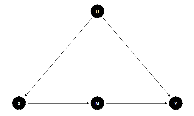
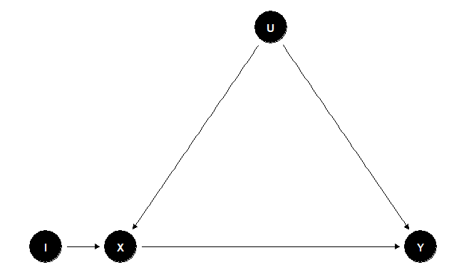
For this criterion, we can find a set of variables \( M \) that mediate all causal influence of \( X \) on \( Y \), which means that all of the direct paths from \( X \) to \( Y \) pass through \( M \). If we can identify the effect of \( M \) on \( Y \) and of \( X \) on \( M \), then we can combine these to get the effect of \( X \) on \( Y \). The test for whether we can do this combination is the front-door criterion. We say that a set of variables \( M \) satisfies the front-door criterion if (1) \( M \) blocks all direct paths from \( X \) to \( Y \), (2) there are no unblocked back-door paths from \( X \) to \( Y \), and (3) \( X \) blocks all back-door paths from \( M \) to \( Y \). Figure 4 presents an SCM in which all the effect of \( X \) on \( Y \) is mediated by the effect of \( X \) on \( M \). With this configuration, we can obtain the effect of \( X \) on \( M \) the back-door is blocked by the collider \( Y \), and the effect of \( M \) on \( Y \) because we can block the back door controlling by \( X \) with these results, finally we can compute the effect of \( X \) on \( Y \)