ε-Machines

In the last post of this series of methods related to causation and prediction I want to introduce a new concept called ε-Machines. This is the first time I am using the term machines in these posts, basically we can think about machines as graphic representations of processes that show the possible states of a system and how it is possible to move from one state to another (transition).

The derivation and study of these type of machines is part of a field known as computational mechanics. According to Shalizi and Crutchfield (2001) “the goal of computational mechanics is to discern the patterns intrinsic to a process. That is, as much as possible, the goal is to let the process describe itself, on its own terms, without appealing to a priori assumptions about the process’s structure.” It is important to notice that the same term also refers to something different concerned with the use of computational methods to study events governed by principle of mechanics. Knowing that there exist different interpretations for the same concept, in this post, we will focus on understanding how a process computes.

Causal States, Transitions, and ε-Machines

To produce a better explanation of the method I am going to revise the concepts of causal states and transitions (state-to-state) that we need to understand what a causal state machine is.

A causal state of a process is defined as the set of histories that lead to the same prediction. For example, we want to predict Xavier’s emotional expression tomorrow to make the prediction we have two different pasts $\overleftarrow{s'}$ and $\overleftarrow{s''}$ . If the two pasts make the same prediction we say that $\overleftarrow{s'}$ and $\overleftarrow{s''}$ have the same morph. Every causal state has a unique morph. Figure 1 shows an example of two causal states that for the behavior of an automated bot on social media.

Figure 1

From figure 1 we notice that having the causal states determined is not enough to define a process. For causal state machines knowing the causal state at any given time and the next value of the observed process together determine a new causal state. In other words, there exists a natural relation of sucession among causal states. Moreover given the current causal state, all the possible next values of the process have conditional probabilities well defined. Formally, the transition probabilities between states $T_{ij}^{(s)}$ is the probability of making a transition from state $S_i$ to $S_j$ while the next value of the process is $s$ .

To complete the diagram previously introduced in figure 1, figure 2 presents a causal state machine that describe the posting behavior (process) of a bot on social media. We can appreciate that the observed variable in the process is the mention (or not) of the bot. The diagram allow us to know what the next state is going to be given the current state and the value of the observed variable (mention). We also distinguish that this bot always post when it is mentioned, and is always still when not mentioned.

Figure 2

Now that we understand a little more about causal states, transition probabilities, and diagrams let’s introduce the ε-machines. By definition the ε-machine of a process is the combination of the function that transforms histories to causal states with the transition probabilities among them.

Figure 3 shows the diagram of a toy example of an ε-machine. The idea is to try to predict the emotional expression of Xavier on social media based on the history of his posts on the same platform. So the first step we need to take is to collect the past posts of Xavier and measure their emotions. To make easier let’s say that the emotion measured is clasified in positive or negative, with values 1, and 0 respectively. Therefore, we create a time series of values 0s and 1s. Using the structure of the time series is possible to determine the morphs present in the time series and the transition probabilities between them. As previously estated the morphs determine the number of causal states present in the process. Once we have the causal states and the transitions we can create the diagram for the the ε-machine. The example clearly shows that ε-machines only use the information of one time series to predict a future state in the process. Basically, we elaborate a model for the process based on autoregression but without the assumptions we use to develop ARMA or ARIMA models.

Figure 3

It is important to notice that ε-machines are predictive state machines that comply with three optimality theorems that capture all of the process’s properties (1) prediction: a process’s ε-machine is its optimal predictor, (2) minimality: compared with other optimal predictors, a process´s ε-machine is its minimal representation, and (3) uniqueness: any minimal optimal predictor is equivalent to the ε-machine (Crutchfield, 2012).

Analysis

There are different methods to to build ε-machines models from time series such as topological methods (Crutchfield & Young, 1989), state-splitting (Shalizi et al., 2002; Shalizi & Shalizi, 2004), spectral decomposition, etc. However, the most didactical is the method of subtree reconstruction that I will describe in more detail.

We are interested in obtaining the ε-machine of the process from observed empirical data. Let’s say that we collected the following data $110101011011110$ and we decided to analyze the structure considering windows of lenght four. The first would be $\underline{1101}01011011110$ , the second $1\underline{1010}1011011110$ , and so on until the last one $11010101101\underline{1110}$ . If we draw all the possible windows in a tree structure we will find out that some branches never occur like $0000$ so we need to prune them and the final tree that we obtain is reflected in figure 4.

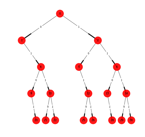
Figure 4

Now that the tree structure is defined we look at the subtree structures that create the building blocks of the process. Considering branches of two steps into the future it is possible to distinguish two different morph which are shown in figure 5a and 5b. The morph of figure 5a can be appreciated in the tree structure of figure 4 starting in the nodes $0$ , $2$ , $4$ , and $6$ while the morph 5b has starting nodes in $1$ and $5$ .

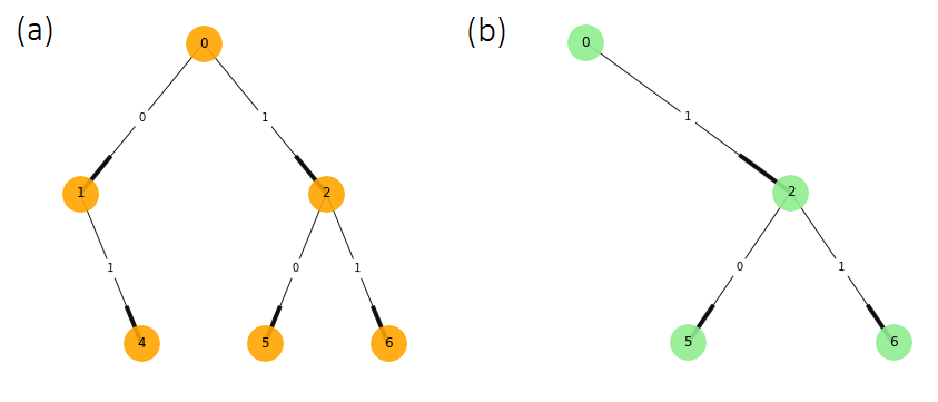
Figure 5

Using the previous morphs as the states of the process and the original tree structure we can define the topological ε-machine shown in figure 6 and its final diagram in figure 7. This model produces strings of data that never contain two consecutive 0s.

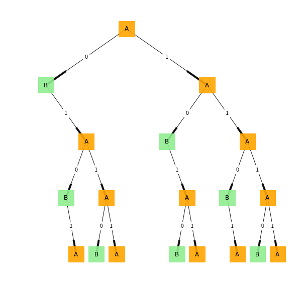
Figure 6

Figure 7

The final model we obtained represents the process topology, in other words, how the different components are arranged. However, it is important to recall that it does not say anything about the probabilities of the occurrences. By counting the frequency of the windows of length four it is possible to provide an approximation of the transition probabilities shown in figure 7. Now, each edge has two numbers now following the format $ed | p$ where $ep$ represents the empirical data observed and $p$ the probability of observing that specific data.

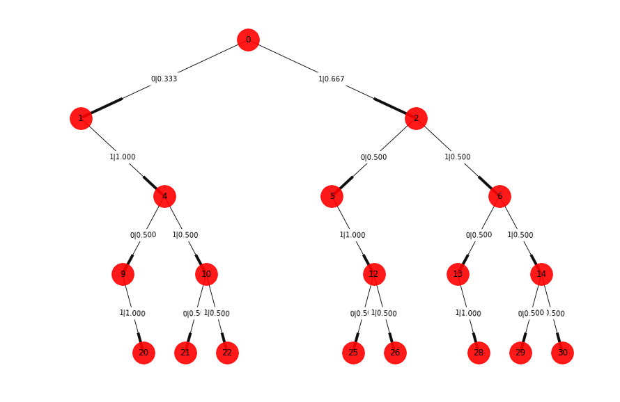
Figure 8

Taking a detailed look of figure 8 we can observe now that we have three different morphs because there is a slight difference in the probabilities between morphs A and C (see figure 9). The new morph creates an initial state represented with the letter A in figure 10.

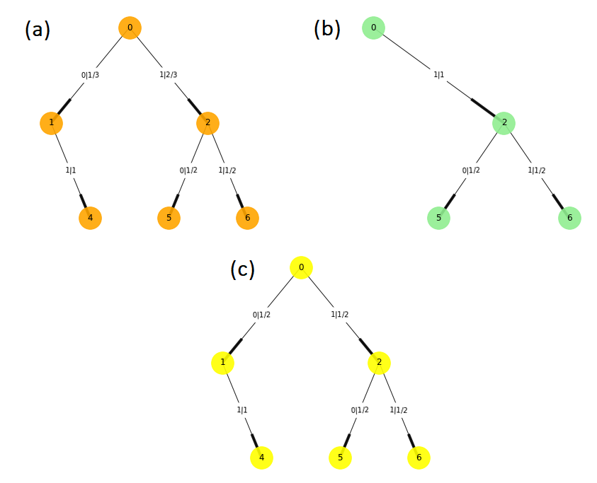
Figure 9

Figure 10

Another important result of having a set of causal states and its probabilities for the ε-machines is that we can compute the information measures for the set of causal states $S$ . The entropy of the states of an ε-machine is called statistical complexity.

(1) $H[S] = C_{\mu}$

Using the definition it is possible to affirm that “the statistical complexity of a state class is the average uncertainty (in bits) in the process’s current state. This, in turn, is the same as the average amount of memory (in bits) that the process appears to retain about the past” (Shalizi & Crutchfield, 2001). In simple, it is the amount of memory about the past required to predict the future.

Limitations

There are different limitations for the use of this tool, it is needed to observe processes that takes on discrete values. The process also is discrete in time variable.

The same as the previous cases of transfer entropy and modes of information flows the observed process must be stationary. The time series is pure which means that it doesn’t have a spatial extent. Finally the predicition is only based on the process’s past, we can’t add any other outside source of information.

References

Crutchfield, J. P. (2012). Between order and chaos. Nature Physics, 8(1), 17–24. https://doi.org/10.1038/nphys2190

Crutchfield, J. P., & Young, K. (1989). Inferring statistical complexity. Physical Review Letters, 63(2), 105–108. https://doi.org/10.1103/PhysRevLett.63.105

Shalizi, C. R., & Crutchfield, J. P. (2001). Computational mechanics: Pattern and prediction, structure and simplicity. Journal of Statistical Physics, 104(3), 817–879.

Shalizi, C. R., & Shalizi, K. L. (2004). Blind Construction of Optimal Nonlinear Recursive Predictors for Discrete Sequences. ArXiv:Cs/0406011. http://arxiv.org/abs/cs/0406011

Shalizi, C. R., Shalizi, K. L., & Crutchfield, J. P. (2002). An Algorithm for Pattern Discovery in Time Series. ArXiv:Cs/0210025. http://arxiv.org/abs/cs/0210025

ε-Machines

Pablo M. Flores

Modes of Information Flow

Transfer Entropy

Instrumental Variables

Structural Causal Modeling

Granger Causality

Prediction and Explanation in Social Sciences: Introducing a Set of Useful Methods.

Social media